Fast-Track Quantum Simulation with Xanadu’s PennyLane Lightning on AMD GPUs
Dec 09, 2025

Quantum hardware is advancing rapidly, but until machines reach hundreds or thousands of reliable qubits, high-performance simulation is essential for building, testing, and optimizing real applications. State-of-the-art simulators capable of handling large-scale circuits let developers get ahead of the hardware and be ready when the technology arrives.
PennyLane's Lightning on AMD GPUs transforms quantum circuit simulation into a high-performance computing pipeline, enabling researchers and engineers to tackle problem sizes previously unfeasible. Pennylane’s Lightning simulator, running on AMD GPU hardware, has been demonstrated at scale on the Frontier Supercomputer —however, expanding access to quantum simulation requires making this software stack available on a broader range of systems.
In this post, we provide an avenue for anyone to try PennyLane on AMD GPUs via the AMD Developer Cloud. We will show how to do it using three methods: Docker, Python wheels, and source code installation, each tailored to different user preferences and needs. By the end, you will be able to run your first Hello World program on AMD hardware and have a development environment to explore more complex PennyLane programs.
Three PennyLane “Hello World” Programs
PennyLane is a Python-based framework for hybrid Quantum-classical computing, supporting Quantum Computing, Quantum Machine Learning, and Quantum Chemistry (among other uses). It provides the necessary mechanisms to build, compile, and analyze quantum algorithms, and to perform operations such as automatic differentiation through interoperability with classical compute frameworks (e.g., JAX and PyTorch).
PennyLane programs can be executed on a variety of target backends. A backend may be a physical quantum hardware device (e.g., Xanadu’s Aurora or IBM Q), or a quantum simulator suite. Lightning, of the latter category, is PennyLane’s quantum simulator suite. It can run on multiple devices (e.g., CPUs and GPUs) with different implementations (e.g., tensor, qubit, and Kokkos).
In this blog, we will use some Hello World Quantum Circuits written in PennyLane and executed on AMD GPUs. In particular, we have the following three different programs. Code segments in this section emphasize circuit creation. We will revisit the code during the execution phase for complete examples.
Bell State Circuit
This circuit is the standard entry point for quantum entanglement. It allows the creation of two entangled qubits. The result state is defined in Figure 1, and the corresponding circuit in Figure 2.
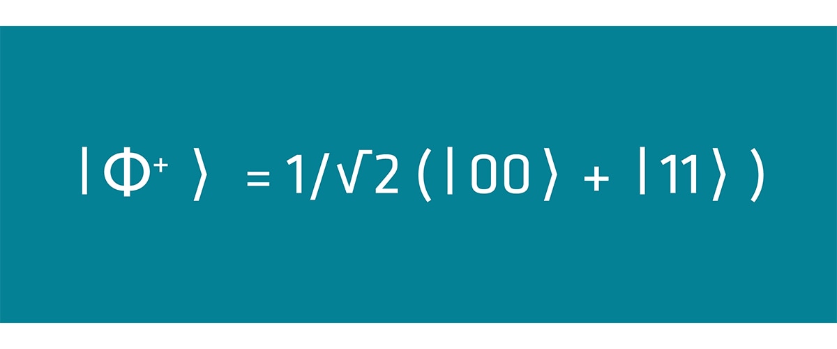
Figure 1: Definition of the Bell state. An equal superposition of ∣00⟩ and ∣11⟩.
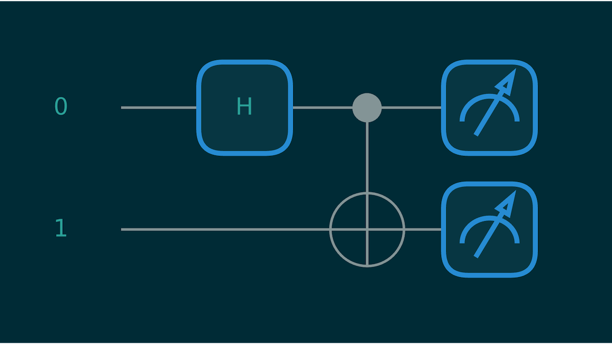
Figure 2: Quantum Bell State Circuit
Expressing this circuit in PennyLane is straightforward, as shown next. We define a circuit via the QNode decorator. A wire refers to a qubit (a horizontal line in the circuit above). For the CNOT gate, the control qubit is the first wire in the list, and the target qubit is the second.
		@qml.qnode(dev)
def circuit():
    qml.Hadamard(wires=0)
    qml.CNOT(wires=[0,1])
    return qml.probs()
Variational Quantum Circuit (VQC)
This example goes a step deeper. Instead of just evaluating a circuit, we benchmark gradient computation for a variational quantum circuit using PennyLane’s StronglyEntanglingLayers template. This type of circuit is common in quantum machine learning because its structure includes trainable gate parameters that can be optimized just like weights in a classical neural network.
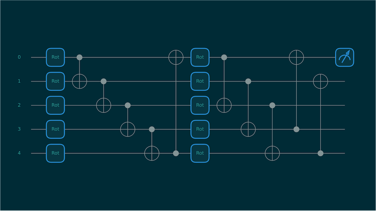
Figure 3: Variational Quantum Circuit for 2 layers and 5 Qubits.
PennyLane makes building these circuits straightforward, and it integrates cleanly with modern ML frameworks. In this example, we construct a VQC, generate random parameters, and then use JAX to compute the vector–Jacobian product (VJP). A VJP is the primitive used by reverse-mode autodifferentiation—essentially the “backward pass” that lets us evaluate gradients efficiently without ever forming the full Jacobian matrix.
		# Create QNode of device and circuit
@qml.qnode(dev)
def circuit(parameters):
    qml.StronglyEntanglingLayers(weights=parameters, wires=range(wires))
    return qml.expval(qml.PauliZ(wires=0))


# Set trainable parameters
shape = qml.StronglyEntanglingLayers.shape(n_layers=layers, n_wires=wires)
weights = jax.random.uniform(key, shape)

# Generate a random cotangent vector (matching output shape of circuit)
key, subkey = jax.random.split(key)
cotangent_vector = jax.random.uniform(subkey, shape=())


# Define VJP wrapper
def compute_vjp(params, vec):
    primals, vjp_fn = jax.vjp(circuit, params)
    return vjp_fn(vec)[0]


# JIT the VJP function
jit_vjp = jax.jit(compute_vjp)

vjp_res = jit_vjp(weights, cotangent_vector).block_until_ready()
Here, JAX traces the circuit once, compiles the backward-pass rule, and then executes a fast VJP evaluation. This is the same mechanism that powers backpropagation in classical deep learning, but applied to a quantum circuit. It gives us a realistic picture of gradient performance on both CPU and AMD GPU simulators without drowning in full Jacobians.
Quantum Fourier Transform (QFT)
This final circuit corresponds to a benchmark that runs QFT. This circuit acts as a “heavy” workload, stressing the simulator. An extensive description of this algorithm is available in the Intro to Quantum Fourier Transform tutorial on the PennyLane website.
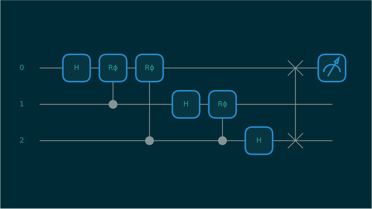
Figure 4: Circuit diagram for a 3-qubit circuit that computes the Quantum Fourier Transform
Another circuit of interest directly supported by PennyLane is QFT. Below, we observe how simple it is to create a QFT circuit:
		@qml.qnode(dev)
def qft_circuit():
    qml.QFT(wires=range(n_qubits))
    return qml.expval(qml.PauliZ(0))
Three Possible Avenues
We understand that developers have different needs and working environments. Therefore, we present three alternatives, each with a different workflow in mind: Docker and Python pip install for fast deployment, and building from source for more control or to develop new features.
Running on AMD Developer Cloud
AMD Developer Cloud is a resource that allows developers and open-source software contributors access to the AMD Instinct™ MI300X GPUs hosted on Digital Ocean. It offers a pay-as-you-go option and functions as a traditional cloud provider for AMD hardware. Additionally, complimentary hours are available for qualified developers.
Running on AMD Developer Cloud is relatively simple. If you have experience with Digital Ocean’s terminology, you will find this process straightforward. Once you sign up, we will create a GPU Droplet with the “Create” menu on the top header bar:
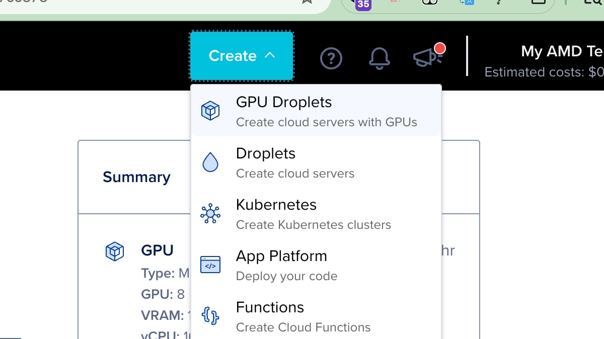
Figure 5: Selection menu “Create” in DevCloud located in the top-right website header. Use GPU Droplets to get access to AMD MI300 Instinct
We select the AMD Instinct MI300X GPU plan and use the Quick Start image that comes preloaded with AMD ROCm™ 7.1 Software. Note that you may request "complimentary cloud hours" and if approved, they will show on your "create droplet page".
Image Zoom
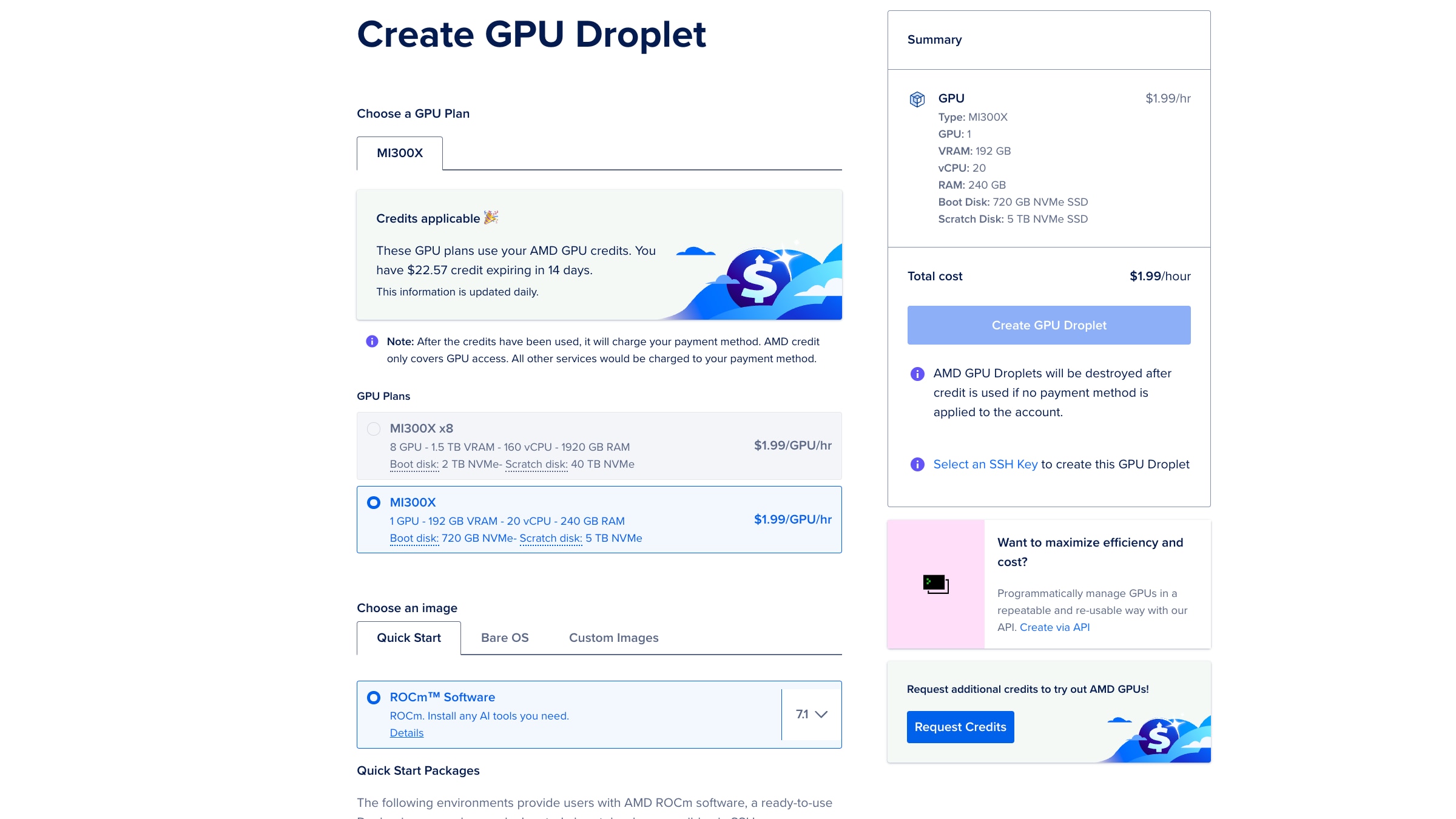
Figure 6: Screenshot of the Droplet creation menu. For this Hello World tutorial, we recommend using a single MI300X, and the preloaded ROCm Software image.
Finally, we will need to add an SSH key and click on the “Create GPU Droplet” button in blue on the right column.
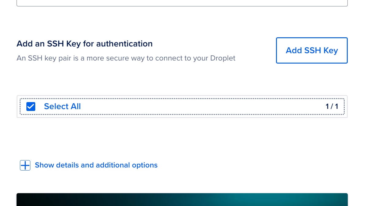
Figure 7: Before creating the droplet, an SSH key must be added and selected.
Once deployed (it may take a few minutes), you can access the droplet via SSH, using the SSH key configured in the previous step and the root user, or via a Jupyter Server that is automatically deployed.
Instructions to access the Jupyter Server can be easily obtained by accessing the Web Console on the top right of the Droplet info:
Image Zoom

Figure 8: GPU Droplet control panel. Use the Web Console at the top right for quick access to the terminal. Public IP, along with other configurations, can be found here.
This will open a new browser window with a terminal. Search for the "Access the Jupyter Server" section, as shown below.
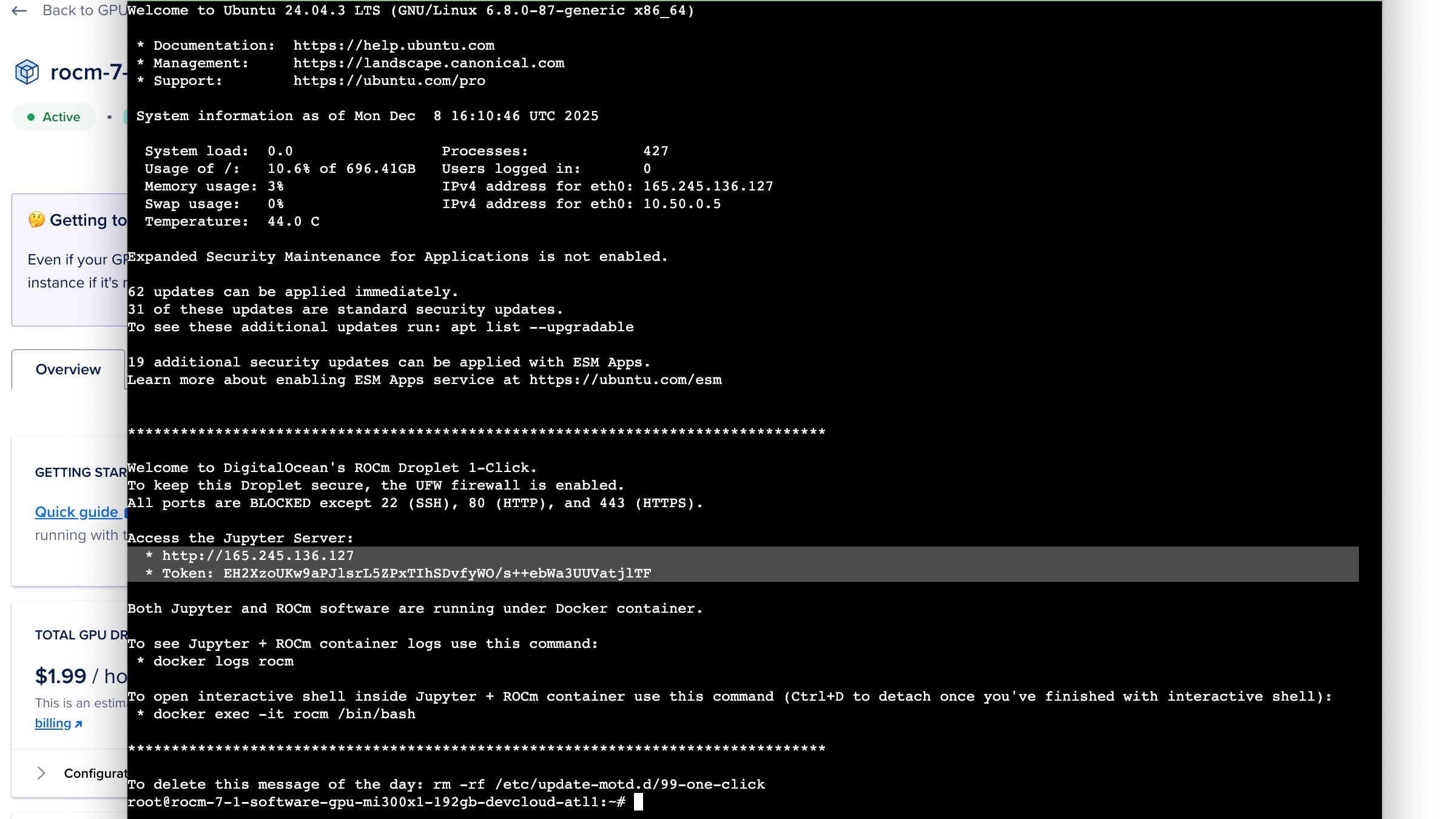
Figure 9: Information displayed upon accessing the Droplet’s Terminal. Follow the instructions in the highlighted area to access the Jupyter Server via the browser.
The Jupyter server is exposed via the droplet's public IP address on the HTTP port. This is accessed via http://<publicIP> in the browser. The home page will have a single input for the token provided above.
Now we’re ready to run PennyLane:
Fetching the examples:
Note: In the Jupyter Notebook, you may need to install git as some images come without it. You can open a terminal (or a code cell in Jupyter), and run apt-get install git
First, we will obtain the three different examples we would like to run.
> git clone https://github.com/PennyLaneAI/amd-devcloud-tutorial.git
Installing or Building PennyLane Lightning
Pip
Open a terminal, or create a Jupyter notebook code block, and type:
pip install pennylane-lightning-amdgpu
Docker
Note: This approach only works from SSH. Jupyter Server runs in its own Docker container, so it does not allow running another container inside it.
Open an SSH terminal (Or the Web Console as instructed above), and type:
docker run -it --device=/dev/kfd --device=/dev/dri --group-add video --rm -v $(pwd):/io pennylaneai/pennylane:latest-lightning-kokkos-rocm /bin/bash
From Source
For full details, see the documentation: PennyLane-Lightning Build Guide
Install dependencies:
sudo apt install cmake ninja-build gcc-11 g++-11 -y
Install Kokkos
Note: This compilation command is for GFX942, the target backend used in MI300X. If building from another architecture, make appropriate modifications. You can check the Kokkos documentation for more information, and get your target backend with the rocminfo
		wget https://github.com/kokkos/kokkos/archive/refs/tags/4.5.00.tar.gz
tar xvfz 4.5.00.tar.gz
cd kokkos-4.5.00

export KOKKOS_INSTALL_PATH=$HOME/kokkos-install/4.5.0/GFX942
mkdir -p ${KOKKOS_INSTALL_PATH}

cmake -S . -B build -G Ninja \
    -DCMAKE_BUILD_TYPE=Release \
    -DCMAKE_INSTALL_PREFIX=${KOKKOS_INSTALL_PATH} \
    -DCMAKE_CXX_STANDARD=20 \
    -DCMAKE_CXX_COMPILER=hipcc \
    -DCMAKE_PREFIX_PATH="/opt/rocm" \
    -DBUILD_SHARED_LIBS:BOOL=ON \
    -DBUILD_TESTING:BOOL=OFF \
    -DKokkos_ENABLE_SERIAL:BOOL=ON \
    -DKokkos_ENABLE_HIP:BOOL=ON \
    -DKokkos_ARCH_AMD_GFX942:BOOL=ON \
    -DKokkos_ENABLE_COMPLEX_ALIGN:BOOL=OFF \
    -DKokkos_ENABLE_EXAMPLES:BOOL=OFF \
    -DKokkos_ENABLE_TESTS:BOOL=OFF \
    -DKokkos_ENABLE_LIBDL:BOOL=OFF
cmake --build build && cmake --install build
export CMAKE_PREFIX_PATH=:"${KOKKOS_INSTALL_PATH}":/opt/rocm:$CMAKE_PREFIX_PATH
Installing PennyLane Lightning
		cd ../
git clone https://github.com/PennyLaneAI/pennylane-lightning.git
cd pennylane-lightning
pip install -r requirements.txt
pip install git+https://github.com/PennyLaneAI/pennylane.git@master

# First Install Lightning-Qubit
PL_BACKEND="lightning_qubit" python scripts/configure_pyproject_toml.py
python -m pip install . -vv

# Install Lightning-AMDGPU
PL_BACKEND="lightning_amdgpu" python scripts/configure_pyproject_toml.py
export CMAKE_ARGS="-DCMAKE_CXX_COMPILER=hipcc \
-DCMAKE_CXX_FLAGS='--gcc-install-dir=/usr/lib/gcc/x86_64-linux-gnu/11/' \
-DENABLE_WARNINGS=OFF"
python -m pip install . -vv
Running our Hello World Programs
Once we have the repository, running these programs is as simple as calling Python. Let’s take a look at the expected outputs:
Bell State Circuit
		> python Example0_Hello_World_Bell_state.py

[0.5 0.  0.  0.5]

0: ──H─╭●─┤  Probs
1: ────╰X─┤  Probs
The result can be interpreted as the following equation, which represents the Bell state.
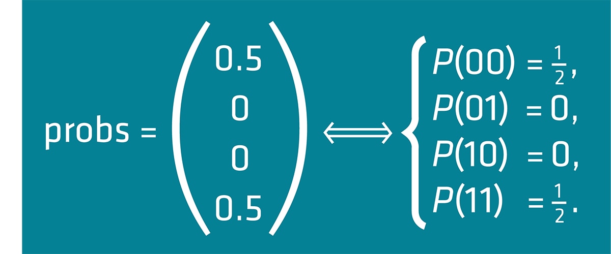
Figure 10: Interpretation of the output probability vectors of Example 0 Bell State.
Also, note that qml.draw(circuit) provides a graphical representation of the circuit we are running.
You can choose the execution device by using “CPU” or “GPU” at the end of the command. For example:
> python Example0_Hello_World_Bell_state.py GPU
Although, for this example we will not notice much difference due to the simplicity of the circuit.
Variational Quantum Circuit
Note: This example requires JAX to run, which can be easily installed via
pip install jax==0.6.2 for PennyLane v0.43, and pip install jax==0.7.1 for the latest PennyLane.
For this example, two parameters can be changed inside the code: the number of wires (i.e., qubits) and the number of layers. We allow the program to print the circuit in two different ways. We run the program using:
> python Example1_BasicEntangling_Gradient.py
But let’s split the output of this program into sections. First, we get the Jacobi measurements of the circuit. This is important when considering Quantum Machine Learning.
		Circuit measurements:
 [0.71853744 0.46851823 0.85051828 0.43891951]
Then it is the raw circuit, which can be obtained via qml.draw(circuit). Notice the use of the StronglyEntanglingLayers as a subcircuit. The drawing will maintain the original hierarchy, providing a valuable resource for understanding the final circuit.
		Raw circuit:
0: ─╭StronglyEntanglingLayers(M0)─┤  <Z>
1: ─├StronglyEntanglingLayers(M0)─┤  <Z>
2: ─├StronglyEntanglingLayers(M0)─┤  <Z>
If we want to observe the actual circuit, we can still use more arguments in the draw function to expand the sub-circuits, such as level='device'. The result is as follows:
		Expanded circuit:
0: ──RZ(0.80)──RY(0.18)──RZ(0.78)─╭●───────╭X──RZ(0.94)──RY(0.00)──RZ(0.99)─╭●────╭X────┤  <Z>
1: ──RZ(0.60)──RY(0.45)──RZ(0.10)─╰X─╭●────│───RZ(0.62)──RY(0.61)──RZ(0.01)─│──╭●─│──╭X─┤  <Z>
2: ──RZ(0.46)──RY(0.33)──RZ(0.14)────╰X─╭●─│───RZ(0.02)──RY(0.52)──RZ(0.40)─╰X─│──╰●─│──┤  <Z>
3: ──RZ(0.65)──RY(0.06)──RZ(0.72)───────╰X─╰●──RZ(0.05)──RY(0.97)──RZ(0.23)────╰X────╰●─┤  <Z>
Finally, we obtain the average execution time over three executions.
Mean timing: 0.08730040066681492
Now that we understand what’s going on, let’s see the GPU in action. We can easily change the device configuration from CPU to GPU using:
		# Use `lightning.qubit` for CPU
# Use `lightning.amdgpu` for AMD GPU
dev = qml.device('lightning.amdgpu', wires=wires)
NowLet’s use these to plot the speedup between the GPU and the CPU for different numbers of layers and wires.
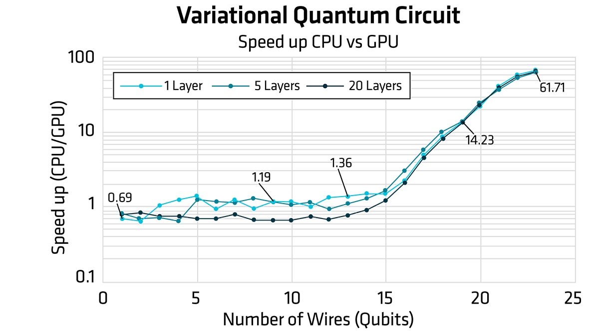
Figure 11: SpeedUp metrics of the VQC circuit training in relation to the number of qubits in the circuit. CPU (lightning.qubit) vs GPU (lightning.amdgpu) for three different numbers of layers.
Quantum Fourier Transform (QFT)
Finally, we can run the Quantum Fourier Transform example. This circuit template in PennyLane is parametrized for the number of wires. Execution is similar to before:
python Example2_QFT.py
It is possible to modify the code to change the number of wires. Furthermore, the device can be set to lightning.qubit for CPU execution, and lightning.amdgpu for GPU execution. Therefore, when varying the number of wires, we obtain the following speed up between CPU and GPU execution.
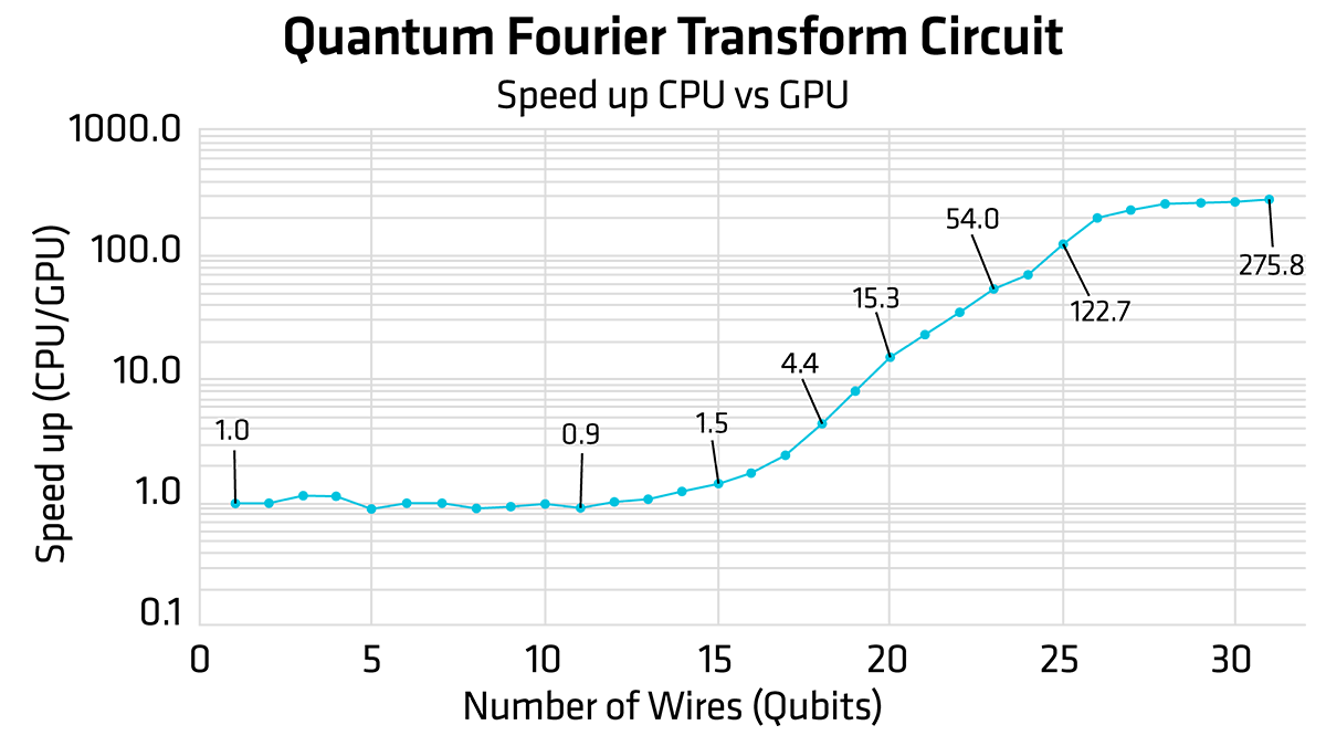
Figure 12: SpeedUp metrics of the QFT circuit in relation to the number of qubits in the circuit. CPU (lightning.qubit) vs GPU (lightning.amdgpu).
Avoid Extra Charges on AMD Developer Cloud
As a user warning, if you are using the Pay-as-you-go option of the AMD Developer Cloud, make sure to delete your droplet after you use it. Droplets that are turned off are still charged at the regular rate. If you want your data or environment to be persistent, there are different approaches to maintaining data, including using Volumes. Refer to the Digital Ocean reference for more information.
Conclusion
As quantum hardware continues to advance toward achieving a large-scale, reliable qubit count, developers can immediately begin exploring quantum algorithms using readily available simulators. AMD GPUs are capable of running cutting-edge quantum software right away. This post illustrates that accessing AMD Developer Cloud allows anyone to start running this software right away. The results presented here demonstrate the importance of GPU acceleration in Quantum Circuit Simulation. Additionally, there are other mechanisms to improve performance (e.g., the Catalyst JIT compilation discussed in Xanadu’s Frontier blog post), which are outside of the scope of this blog post.
If you would like to know more about how AMD is enabling Quantum Computing for the future, do not hesitate to email us at quantum@amd.com
Other Resources
- Expanding the Frontier: Learn how PennyLane and AMD accelerate quantum workflows
- PennyLane documentation - Full guides, tutorials, and API reference
- GitHub Repo - Access all examples and tutorials.
- Xanadu YouTube Channel - Watch hands-on tutorials and deep dives into PennyLane features.
- AMD Developer Cloud - Start projects on AMD Instinct™ GPUs
- PennyLane Lightning GitHub
- The PennyLane Guide to Quantum Machine Learning


Related Blogs
-
Vultr Enables Enterprise AI with Software Components from AMD
Vultr makes AMD Enterprise AI software components available on the Vultr Marketplace, enabling enterprises to run AI at production scale.
June 15, 2026
-
AMD Acquires MEXT to Advance Memory Optimization
Acquisition expands the AMD AI portfolio and helps customers with memory optimization technology
June 15, 2026
-
AMD at Microsoft Build 2026
AMD joined developers, engineers, and AI builders at Microsoft Build 2026 in San Francisco, hosting four hands-on workshops that brought the AMD AI ecosystem directly to attendees
June 12, 2026
-
AMD PACE integrates with vLLM
Run transformer models more efficiently on AMD EPYC™ CPUs with the AMD PACE vLLM plugin and its optimized inference backends.
June 11, 2026
-
How to Check Power Status of a Remote Computer Using DASH CLI
Install and use DASH CLI to remotely query the power state of AIM-T–enabled AMD PRO systems via out-of-band management
June 02, 2026
-
Adapting AIM LLMs For Specific Use Cases Through Fine-Tuning in AMD AI Workbench — ROCm Blogs
Learn how to adapt and fine-tune an AIM LLM in AMD AI Workbench GUI for specialization or specific use cases.
June 02, 2026
-
AMD Silo AI & Delphyr AI Collaborate to Scale Practical Clinical AI
AMD Silo AI and Delphyr AI deliver scalable, privacy-first clinical AI: faster EHR retrieval, high-performance embeddings, and seamless workflow integration.
June 02, 2026
-
Accelerating Applications with AOCL Cryptography
See how AOCL Cryptography boosts performance critical applications: ClickHouse, strongSwan, and RocksDB with faster encryption on AMD Zen™ based microarchitecture.
June 02, 2026