Designing Resilient Routing using Quantum Algorithms with Classiq and Comcast on AMD GPUs

Introduction

Modern telecommunications networks employ dense graph topologies in which multiple physical paths exist between any pair of sites. This redundancy provides crucial resilience: when a link fails along one path, traffic can be re-routed through backup paths to maintain service continuity. However, fully leveraging this built-in resilience requires algorithms that can optimize for multiple competing objectives simultaneously—such as minimizing latency while avoiding correlated link failures (example, links that may fail together due to shared environmental hazards).

Finding optimal paths under these constraints is computationally challenging. The problem of identifying disjoint paths that simultaneously minimize latency and dual link failure risk is NP-hard, meaning classical algorithms struggle to find optimal solutions as network size grows. This is where quantum computing offers a promising alternative. In this blog, we formulate the latency-resilient routing problem as an optimization task and demonstrate how quantum algorithms can tackle this computationally difficult challenge. We present results from executing our quantum algorithm on a GPU-based quantum simulator, thereby showing how quantum approaches may enable telecommunications providers to achieve better routing decisions in increasingly complex networks.

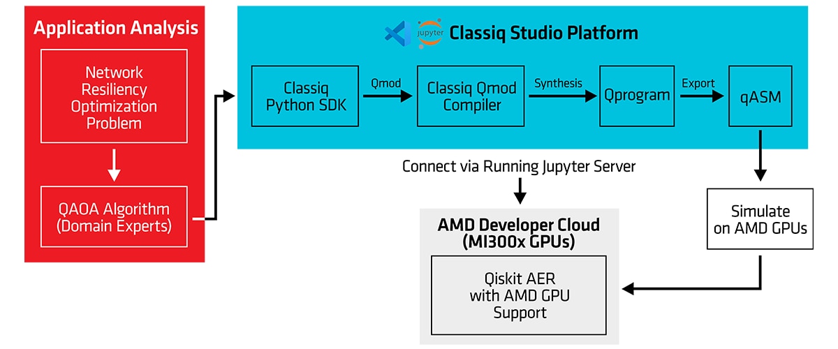
Figure 1 presents an end-to-end flow diagram illustrating the process described in this blog. On the left, we present application analysis, in which we take an algorithm from an application (e.g., binary decision variables for a network resiliency optimization problem) and adapt it to Quantum Computing via the Quantum Approximate Optimization Algorithm (QAOA) design pattern. We then use Classiq’s studio platform to write a high-level program using the Classiq Python SDK. As we will observe, application developers do not write the quantum circuit themselves. Instead, the SDK program is compiled into Qmod, a language that can be synthesized into the resulting quantum circuit, enabling optimizations to be applied to the final circuit. Once synthesized, the circuit can be exported to a lower-level circuit representation for either physical qubits (on actual quantum computers) or simulated qubits. In this case, we use the Qiskit Aer simulator, running on AMD Instinct™ GPUs  via AMD Developer Cloud, to evaluate the resulting quantum circuit.

Problem Statement and Mathematical Formulation

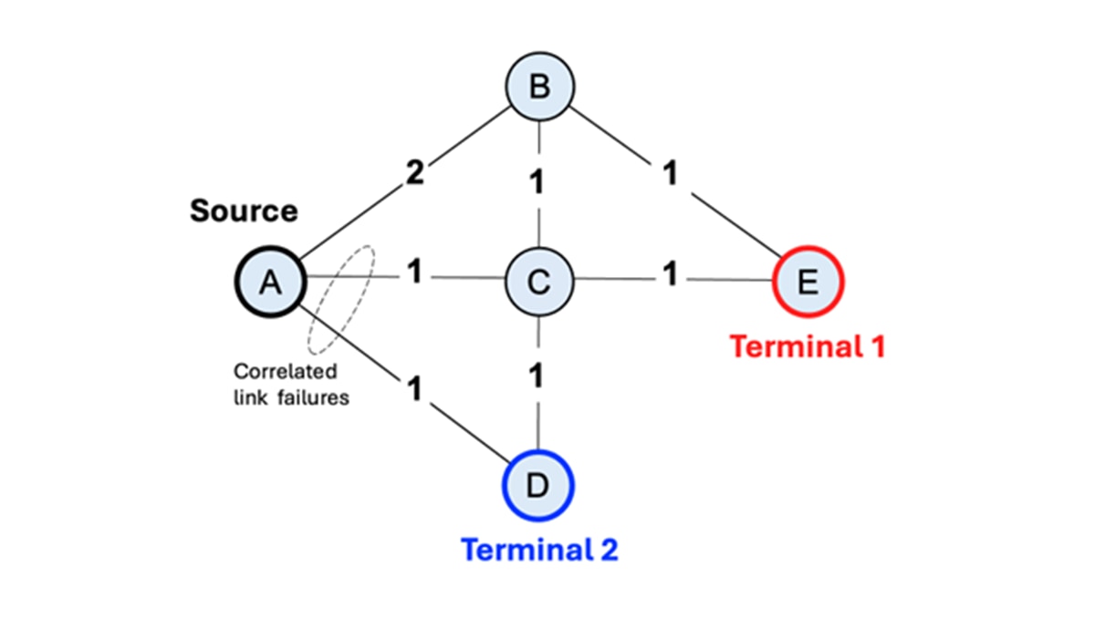
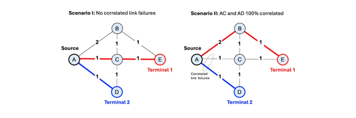
Consider the graph shown in Figure 2 above. Each vertex represents a site serving thousands of Internet subscribers, while edges represent physical links (typically, optical fibers) connecting these sites. The label on each edge indicates link latency in arbitrary units. Vertices D and E are special sites that connect to the Internet backbone. We call these “terminal sites”.

Our objective is to find two disjoint paths from each source site (e.g., site A) to terminal sites D and E: a primary path and a backup path. Disjoint paths share no common edges or vertices, ensuring that a single link or site failure cannot disrupt both paths simultaneously. Additionally, we want to minimize total path latency (the sum of edge weights) while avoiding highly correlated links (more on this later). This is a challenging combinatorial optimization problem: for each source site, we must select two paths from an exponentially large solution space while satisfying hard constraints (vertex disjointness) and optimizing multiple objectives (latency and impact of dual link failure).

Graph optimization problems of this type can be mathematically modeled using binary decision variables. At the core of our problem is finding two shortest disjoint paths: path P1 from site A to terminal D, and path P2 from site A to terminal E. Each path requires a number of binary decision variables equal to the sum of the number of vertices and the number of edges in the graph.

For example, binary decision variable x_ij^P1 equals 1 if edge (i,j) is active (i.e., is part of the path from A to D), and 0 otherwise. Similarly, variable x_i^P1 equals 1 if vertex i is active (i.e., part of the path from A to D), and 0 otherwise. Therefore, the total number of variables needed to model the problem for source site A is 2(|V|+|E|) = 24.

We may express latency minimization using the following objective function:

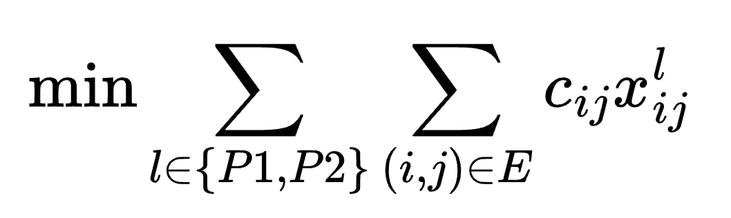
where c_ij represents the latency of edge (i,j). However, you can immediately see the problem: minimizing this objective alone produces a trivial solution where no edges are included in any path—giving zero latency but also zero connectivity! To ensure that only valid paths are returned, we must add path connectivity constraints that force the solution to represent actual routes from source to terminal. Path connectivity is encoded using the following expression:

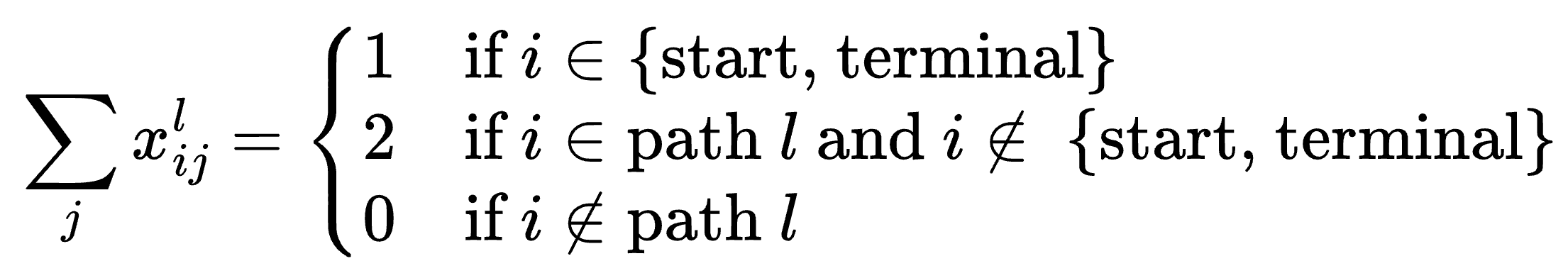
The expression above states the following: a vertex that is part of path P has either 1 active edge (if vertex is the source or terminal site) or 2 active edges (if vertex is an intermediate site). Alternatively, a vertex that is not part of path P has 0 active edges. 

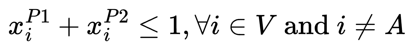
The next constraint enforces path disjointness. That is, P1 and P2 must have no common vertices aside from the source vertex A. By extension, two paths that have no common vertices also have no common edges. Path disjointness is expressed as:

Lastly, we need to penalize having two correlated edges, each being part of paths P1 and P2. Notice that ignoring link correlations gives a false sense of resilience: while P1 and P2 appear redundant on the graph, in reality, they may be including links that are susceptible to the same types of hazards. We will consider the simple scenario in which edges AC and AD are 100% correlated and all other pairs of edges in the graph share no common risk. The following expression is added to the objective function: 

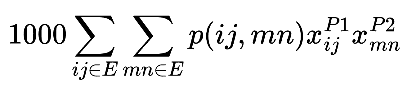
The dual link failure probability, p(ij,mn),  is 0.1 only if edges (i,j) and (m,n) correspond to AC and AD. Otherwise, p(ij,mn) takes the value of 0.01. The scaling factor 1000 is purposely chosen to be much larger than edge weights, so that avoiding correlated link failure takes precedence over minimizing latency. 

We have now encoded the problem using a combination of to-be-minimized objective function and some constraints! Note that in order to solve the problem using quantum algorithms, we need to combine the objective function and constraints in a single expression. This straightforward step is not covered in the Blog but can be referred to in the accompanying publication^[1].

Quantum Approximate Optimization Algorithm (QAOA)

Thus far, the problem was formulated mathematically using a single objective function that encompasses both the optimization goals and necessary constraints (incorporated as penalty terms). This unified expression is called the Hamiltonian - a foundational concept from physics representing the energy landscape and interactions within a system. In physics, the Hamiltonian governs how systems evolve over time, and we leverage this same principle here: by encoding our combinatorial optimization problem as a Hamiltonian, we can harness quantum hardware to evolve a physical system of quantum particles toward the solution of the problem.

To solve this quantum-encoded problem, we use the Quantum Approximate Optimization Algorithm (QAOA), a hybrid approach that combines the strengths of both classical and quantum computing. Think of QAOA as a sophisticated search method where classical computers handle the computational heavy lifting - calculating objective functions and checking constraints - while quantum processors explore the vast landscape of possible solutions in ways impossible for classical machines. The algorithm works by alternating between two types of operations: the problem Hamiltonian (encoding what we’re trying to solve) and the mixer Hamiltonian (exploring different solution candidates). These operations are applied sequentially in layers, with each layer bringing us closer to high-quality solutions. The key challenge lies in tuning the parameters that control these operations, a task handled by classical optimization, to maximize confidence in the solution quality. 

Mathematically, this process is achieved by starting with the so-called uniform superposition state:

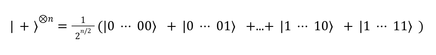
in which every “scenario” (namely, a state within the space of 2ⁿ possible states of the system) is represented with equal probability. Then, a parametric circuit implementing the following action is applied to the uniform superposition state:

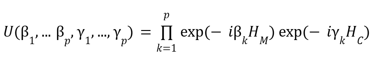
Here, p is the number of QAOA layers, β_k,𝛾 _k the parameters of the circuit, which undergo classical optimization at each iteration of run and measurement of the circuit, and H_C,H_M are the cost and mixer Hamiltonians, respectively. The operation of this circuit structure demonstrates the unique power of quantum computing, where the wavefunction of the qubits undergoes a carefully-designed process of destructive interference to eliminate the undesirable states from the initial collection of all possible states of the system.

The process goes as follows: the objective function is encoded into the cost Hamiltonian, such that throughout the application of the circuit, states which are less favored (namely, have a larger cost) are penalized by accumulating larger phases under the unitary evolution exp(- i𝛾 H_C). The interference of different states is then facilitated by the application of the mixer layer, allowing amplitudes - and thus, probabilities of experimental outcomes - to ‘flow’ between states, amplifying low-cost states while stifling high-cost ones. At each run + measurement iteration of the circuit, the state is further optimized to favor lower-cost states by plugging the measurement result into a classical optimizer and adjusting β_k,𝛾 _k accordingly.

We implemented the algorithm using the Classiq platform described in the subsequent section. The Classiq platform allows researchers to write quantum programs using familiar Python syntax rather than wrestling with low-level quantum gates. The algorithm runs the quantum circuit multiple times, measuring the results and selecting the best solution found. While QAOA does not guarantee perfect solutions, it can be competitive with classical approaches for certain optimization problems, and as quantum hardware continues to improve, its advantages will only grow.

Classiq QMOD

Quantum computing development is hindered by the low-level complexity of circuit design. Classiq solves this with a high-level Domain-Specific Language (DSL) called Qmod, as well as a powerful quantum compiler. 

The High-level language allows developers to describe the logic of the quantum algorithm concisely. The compiler then autonomously synthesizes and optimizes the most efficient quantum circuit.

This approach ensures:

1. Scalability: Handles the exponential complexity growth for large problems.
2. Ease of Use: Lowers the barrier for non-specialists to utilize quantum hardware.
3. Efficiency: Generates smaller, shallower circuits that are more robust to noise.

Classiq’s high-level language and compiler are essential tools for tackling complex, NP-hard problems, making the transition from mathematical problem to executable quantum circuit simple and scalable.

Note that developers do not need to write Qmod if they prefer to use Python. Classiq provides a Python SDK that allows Qmod programs to be created via decorators and other APIs. This will be demonstrated below.

Simulation Infrastructure Setup in DevCloud

We aim to demonstrate that our AMD GPU infrastructure can be used with Classiq. Thus, we use AMD Developer Cloud to create an environment with MI300x GPUs that serves as the execution backend for Classiq’s Studio Platform. In this section, we describe how to set up AMD Developer Cloud and build Qiskit-AER with AMD GPU support. 

Creating a droplet

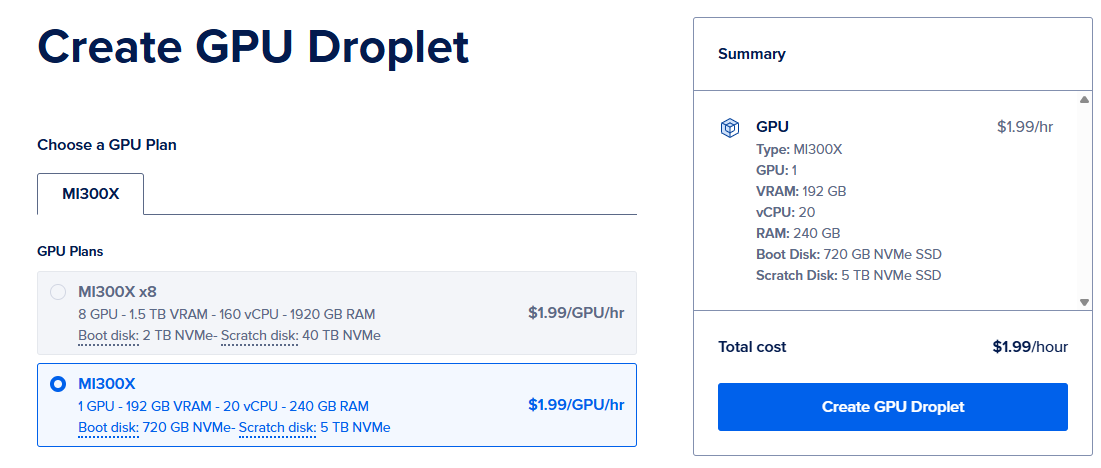
Assuming that you already have an account (anyone can create one at https://amd.digitalocean.com/login), you will need to create a new droplet. A droplet is the DigitalOcean term for a virtual machine. To achieve this, we can use the Create menu in the top-right corner of the website, as shown in Figure 4. We select GPU Droplets.

There are two flavors of GPU Droplets that differ in the number of GPUs allocated: MI300X (1 GPU) and MI300X x8 (8 GPUs). Be aware that cost is proportional to the number of GPUs; therefore, MI300X x8 will be 8 times more expensive. 

For the work performed in this blog post, we will use a single GPU, as shown in Figure 5. We encourage users to test the MultiGPU support available in Qiskit AER.

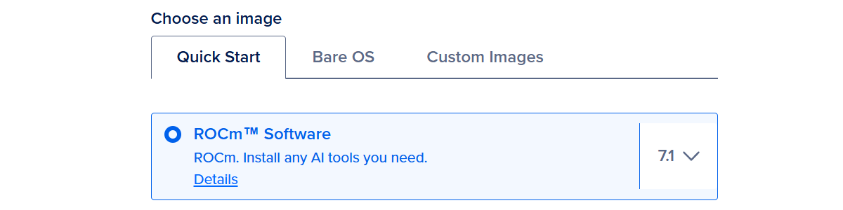
In addition to selecting the number of GPUs, we must select an operating system image used to boot up the virtual machine. Among the available options, we will use the plain AMD ROCm™ software image, as shown in Figure 6.

Finally, we will need to add an SSH key, as shown in Figure 7. This is useful for SSH connections; however, in this example, we will use the preloaded Jupyter notebook environment. Therefore, no SSH connection will be required.

Once we’re ready, we can click on the Create GPU Droplet button. This process may take a couple of minutes while the virtual machine is commissioned. Once created, you will see a droplet control panel similar to that presented in Figure 8.

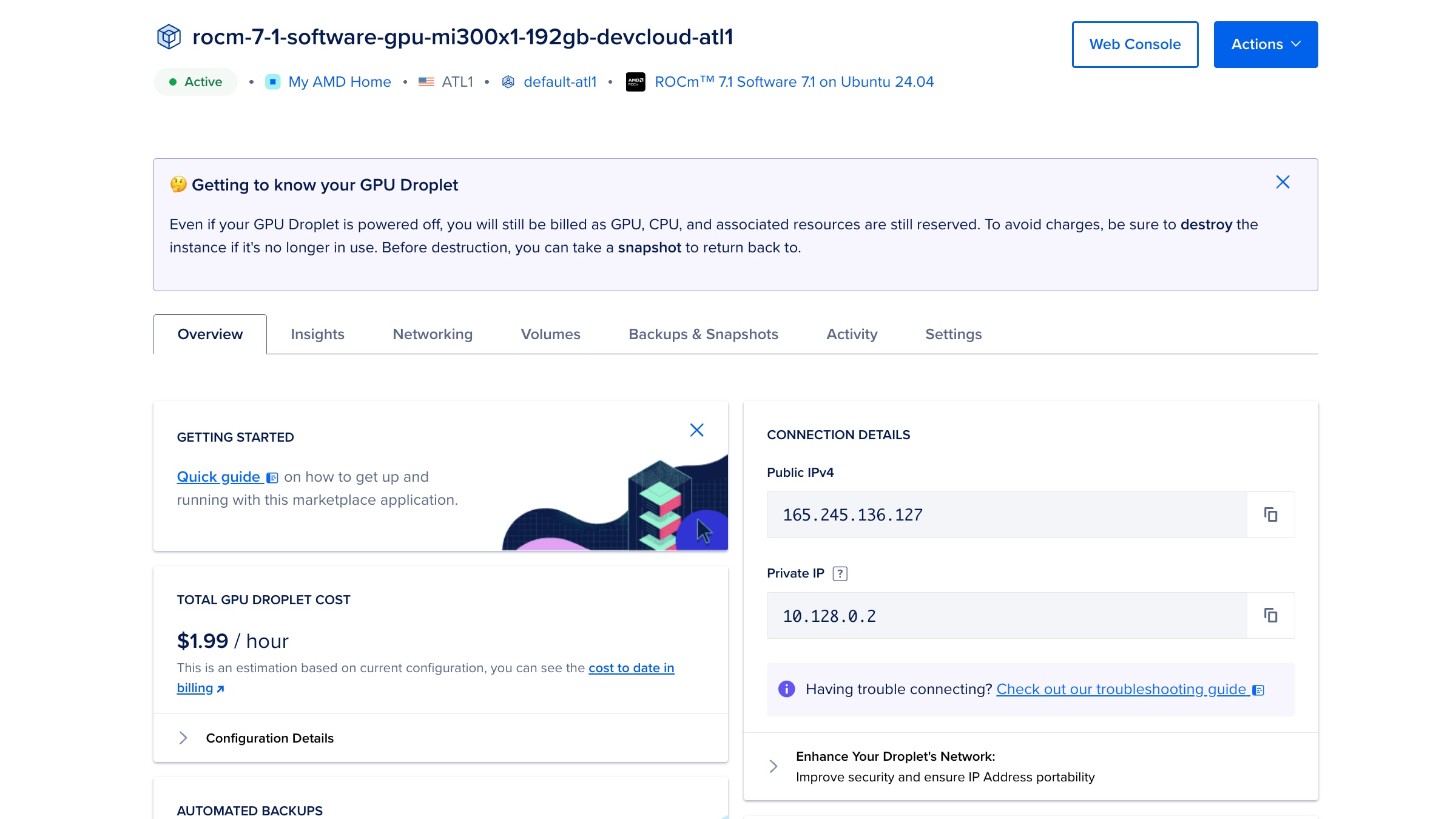
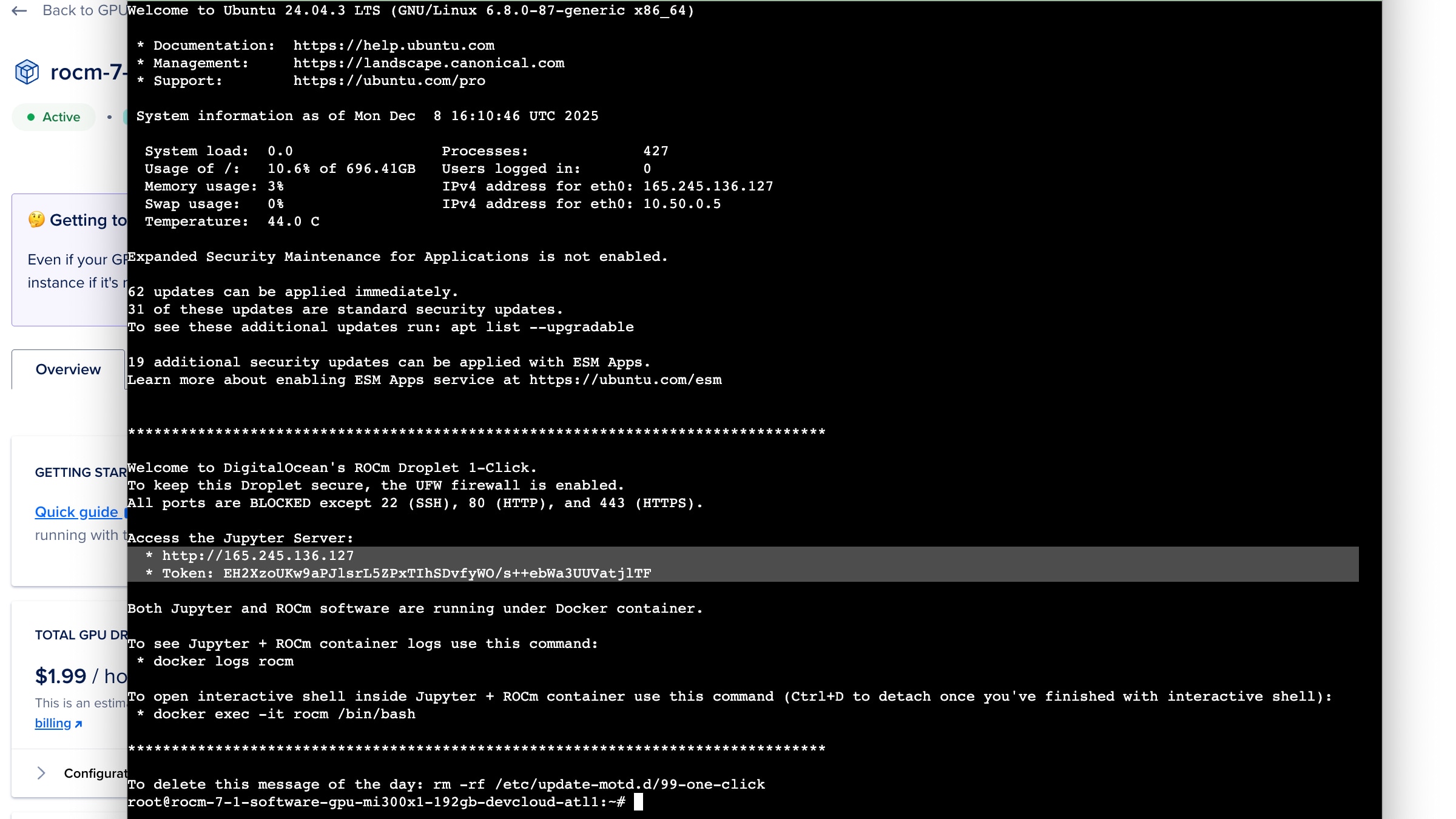
The final step in this process is to learn how to access the Jupyter notebook environment to set up Qiskit-AER and connect from the Classiq studio platform. To do this, we can use the Web Console white button, as shown in the top-right corner of Figure 8, to open a web-based terminal. Figure 9 shows an example of the output you will see after opening the terminal. The two lines after “Access the Jupyter Server” are the important ones. We can open the HTTP address in any browser and use the token to log in, once prompted.

Building Qiskit-AER for AMD GPUs

Now that we have our execution environment ready, it is time to build Qiskit-Aer. We will use a fork of Qiskit-AER that is currently under review for merging into the main project. We will be using the 0.17.2-amd-rocm-dev tag for this blog post.

The following instructions have been added to the preloaded Classiq Jupyter Notebook, which is described below. For completeness, the following are the instructions we use to build Qiskit-AER on DevCloud.

We’re now ready to use the AMD GPUs and Qiskit-AER inside the Classiq Studio Platform.

Classiq Studio Platform

Classiq offers different ways of programming high-level programs. One of the most commonly used platforms of quantum programming with Qmod is using the Classiq Studio, which is a hosted Visual Studio Code-based environment specifically designed for programming Classiq. This allows users to also leverage Classiq’s unique AI coding assistant, specifically designed for programming using the Classiq SDK. 

It is very common to use Jupyter Notebooks for programming various algorithms. Here, the Classiq Studio has specific elements for circuit execution and visualization. This allows users to stay in the Studio while inspecting their created circuits. Making this the perfect single developer experience for any quantum developer.

It is easy to leverage the power of AMD GPUs inside the Classiq Studio. When a GPU instance is set up in the DevCloud, a Jupyter Notebook server runs by default. In the Classiq IDE, it is straightforward to connect to an external Jupyter notebook server, enabling easy access to the AMD GPU instance running in the DevCloud.

We assume you have an active Classiq account with access to Studio. On the classiq.io website, we open Studio by selecting the first menu item on the left, as shown in Figure 10.

This will open a new browser window. After a few minutes, you will be redirected to a website hosting a Visual Studio IDE. The file explorer is divided into two sections, as seen in Figure 11. The Classiq Library is a read-only section that contains a large set of preloaded resources, including Classiq’s examples and tutorials. The notebook used in this blog post is located at Classiq Library > applications > telecom > resiliency_planning > resiliency_planning_AMD.ipynb. The User Workspace supports persistent user data that remains available across sessions. We recommend copying the Jupyter notebook to your User Workspace to enable further exploration before setting up the execution environment. As a side note, the notebook is also available in Classiq’s library repository.

In the workspace area, a Jupyter notebook environment will launch. We need to switch the execution kernel to use the remote Jupyter server located at the AMD Developer Cloud. This is accomplished by clicking on Select Kernel in the upper right corner of the Jupyter notebook interface, as illustrated in Figure 12.

From the pop-up menu, select Existing Jupyter Server (refer to Figure 13). Proceed to follow the instructions, utilizing the HTTP URL provided by the AMD Developer Cloud previously, along with the corresponding access token. Note that this is the same access token used to initially access the Jupyter notebook via your browser.

With our setup complete, we can now run the Classiq Jupyter notebook directly on the AMD Developer Cloud GPUs. This configuration is essential for leveraging the full capabilities of the Classiq SDK and platform tools while executing on a dedicated, AMD powered server with the Instinct GPUs. 

Code Structure and Execution

Writing the Qmod code to generate the quantum circuit is very straightforward. Classiq’s Python SDK allows users to write the objective function in plain Python without any quantum-specific constructs.

This is the pure Python objective function; all the functions that are called in this function can be found in the full notebook:

One of the most important points in the QAOA circuit is the ansatz, this ansatz encodes the cost_hamiltonian(), into a quantum circuit. With Classiq, creating this quantum circuit is very simple. The code below creates the quantum circuit from the Python objective function.

To create the QAOA circuit, we can synthesize the high level code into a circuit using the synthesize() function, like this:

The qprog variable now has the low level quantum circuit representation of our program, this includes a QASM circuit. This QASM circuit can be used to execute the circuit on the AMD GPUs. The flow of the execution looks like this, some details have been left out and can be seen in the full notebook:

Finally, the transpiled circuit can be executed like this:

Once we have a circuit and execute the final part of the algorithm is the hybrid execution. The QAOA circuit has multiple parameters; the goal of the hybrid flow is to determine parameter values that yield the correct solution to the problem. To do this, we will start with a simple set of parameters and tune them at each step, as discussed previously. To run this optimization loop, SciPy is used to minimize the Hamiltonian's cost. To make this work, we first need a way to get the cost of each iteration. To do so, we use this function:

Before we can run the minimization, we need an initial set of parameters, which are calculated like this:

Now that there is a way to execute the code on the AMD GPU, we have initial parameters, and we have a way to determine the cost for each run with a specific set of parameters. It is time to tune the parameters. Which can be done like this:

Once this completes, the optimization_res variable should hold the optimal parameter values.

The full code is provided in the notebook.

Results and Discussion

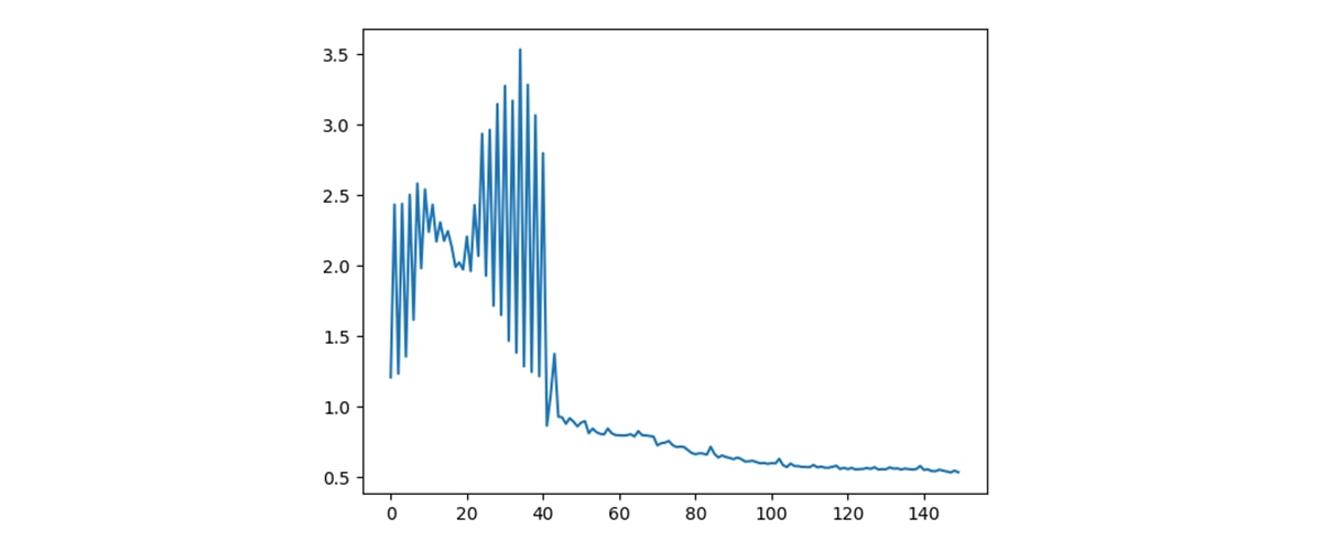
Once the optimal QAOA parameters are identified through the classical optimization loop, we execute the circuit with those parameters to obtain candidate routing solutions. As shown in Figure 14, the hybrid optimization procedure steadily reduces the value of the cost Hamiltonian over successive iterations. After an initial exploration phase with noticeable oscillations, the cost converges to a stable minimum. This behavior reflects the interplay between the mixer and cost layers in QAOA, in which successive parameter updates increasingly bias the quantum state toward configurations that satisfy flow conservation, disjointness constraints, and correlated-link penalties while minimizing total latency.

We evaluated the algorithm on the two scenarios described earlier. In Scenario I, where no link correlations are present, the simulation returns the pair of shortest vertex-disjoint paths from the source to the two terminals, minimizing total latency while satisfying all constraints. In Scenario II, where edges AC and AD are fully correlated, the optimizer avoids selecting both edges simultaneously, even though they may appear attractive from a pure latency perspective. Instead, the returned solution reroutes one of the paths to eliminate correlated risk, demonstrating that the penalty term embedded in the Hamiltonian effectively reshapes the energy landscape. In both cases, the most frequently sampled bitstrings correspond to valid, constraint satisfying flows, confirming that the QAOA circuit successfully encodes both the optimization objective and the structural requirements of the routing problem.

The two solutions visualized in Fig. 15 for the corresponding dual-link failure scenarios were both returned by QAOA as the highest-frequency solutions (~1% probability). Note that 1% is considered a strong signal given that the search space contains 2²⁴ combinations. 

Beyond these illustrative examples, the simulation framework supports scaling to larger graph instances. The high-performance AMD cards enable the execution of very large quantum circuits on a single card due to their large VRAM. This enables rapid, large-scale runs, which are ideal for hybrid scenarios like this. By leveraging AMD GPU acceleration within the simulator, we can increase the problem size to 7-node configurations, with one source node and two terminal nodes that require up to 32 qubits. While these larger instances are not shown here, this capability demonstrates that the combined high-level modeling in Classiq and GPU-accelerated statevector simulation enables exploration of substantially larger solution spaces than would otherwise be practical in a purely CPU-based environment.

Conclusion

This blog post presented a complete, real-world application workflow that leverages the Quantum Approximate Optimization Algorithm (QAOA) to solve a Network Resilience problem, executed entirely on AMD GPUs. We first demonstrated the utility of the QAOA design pattern for this specific challenge. Next, we highlighted the ease of implementation on Classiq's platform, including the Classiq Python SDK, QMod, and the Classiq Studio Platform, which enable algorithm realization using simple, high-level syntax. Finally, we demonstrated the capabilities of AMD Instinct GPUs by executing a quantum circuit on their hardware, leveraging their extensive memory capacity to scale to larger qubit counts—a significant advantage over current quantum hardware access limitations. This work serves as an exciting call to action, encouraging exploration of Quantum applications and future preparedness through the combined strengths of Classiq’s advanced software infrastructure and AMD’s powerful hardware.

If you have any questions or would like to learn more, you can contact us at quantum@amd.com, maher.harb@gmail.com