LLM-D Serving for AMD Instinct GPUs on OCI

Introduction

Production LLM serving is ultimately an SLO optimization problem: teams are not simply trying to maximize raw throughput, but to deliver the right latency and responsiveness targets at the lowest possible infrastructure cost. Prefill-decode disaggregated serving with llm-d¹ offers a powerful way to do this, but realizing its benefits requires a disciplined workflow for identifying the right configuration for a given model, workload, and service objective. In this blog, we walk through a practical methodology for tuning PD disaggregated serving to meet inference SLOs efficiently on AMD Instinct™ MI300X GPUs hosted on OCI bare-metal GPUs with a RoCEv2 backend RDMA network.

We begin by benchmarking the major phases of generation independently: decode, prefill, and aggregated serving. By isolating these behaviors, practitioners can better understand the performance envelope of each stage and identify candidate configurations that are well-matched to the model’s compute profile. Rather than guessing at cluster shape or resource ratios, this gives a grounded starting point for configuration selection.

From there, we perform a Pareto sweep across candidate setups to evaluate the tradeoffs between latency, concurrency, and efficiency. This makes it possible to see which configurations are optimal at different load levels, and where the benefits of disaggregation become most pronounced. Instead of a single “best” setup, the result is a decision framework: which PD configuration makes sense for a given concurrency target and SLO requirement.

Finally, we validate the selected configuration with a scale-out run, showing how the methodology extends from single-stage benchmarking to realistic distributed deployment. The result is a repeatable workflow for moving from microbenchmark data to production-ready serving architecture, ultimately helping teams use llm-d to hit inference SLOs with the most efficient prefill-decode configuration possible.

Experimental Setup

Code: https://github.com/tlrmchlsmth/j-pareto

We consider 2 models, an MoE model and a dense model as representative cases of how different model architectures perform with PD disaggregation. We chose openai/gpt-oss-120b and RedHatAI/Llama-3.3-70B-Instruct-FP8-dynamic respectively. These are both popular models for use in enterprise deployments, and are models whose size permit many different parallel configurations, which is needed for disaggregated deployments to show speedup over aggregated ones.

We enable two AMD optimizations for vLLM: AITER unified intention implementation and the quick reduce quantization² optimization.

We use the recommended gpt_oss evaluation scripts from gpt_oss for openai/gpt-oss-120b and lm-evals for RedHatAI/Llama-3.3-70B-Instruct-FP8-dynamic. For convenience, we provide justfile recipes that invoke evaluation here.

All decode benchmarks are using vLLM’s DecodeBenchConnector, a KVConnector that fills the KV cache while skipping the prefill, allowing us to accurately take into account the cost of attention while running pure decode workloads.

Testing was performed on a 72-GPU cluster across 9 Kubernetes nodes deployed on Oracle Cloud Infrastructure (OCI), each configured with 8 MI300X GPUs and 8 RoCEv2-enabled ConnectX-7 NICs.

Why and How to Configure P/D Disaggregation?

Code: j-pareto/pd-config

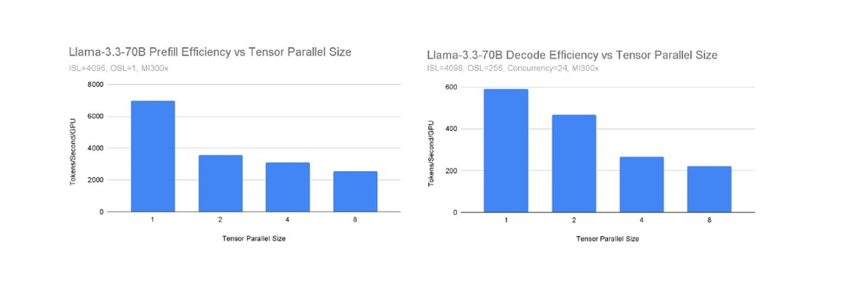
Why to use P/D: The main motivation for prefill-decode disaggregation is it allows specialization between the prefill and decode phases of inference. Prefill is compute-heavy, and a single running request can fully-utilize GPU compute. In contrast, decode is heavy on data movement, and needs a large number of concurrent requests to saturate compute in an LLM’s linear layers, in turn requiring a massive amount of KV cache space. With P/D disaggregation we can parallelize the prefill and decode phases differently. In the below charts, we compare vLLM’s prefill efficiency to its decode efficiency in terms of tokens per second per GPU as we vary the tensor parallel size while serving Llama-3.3-70B. Clearly, decode performance falls off much more slowly than prefill performance.

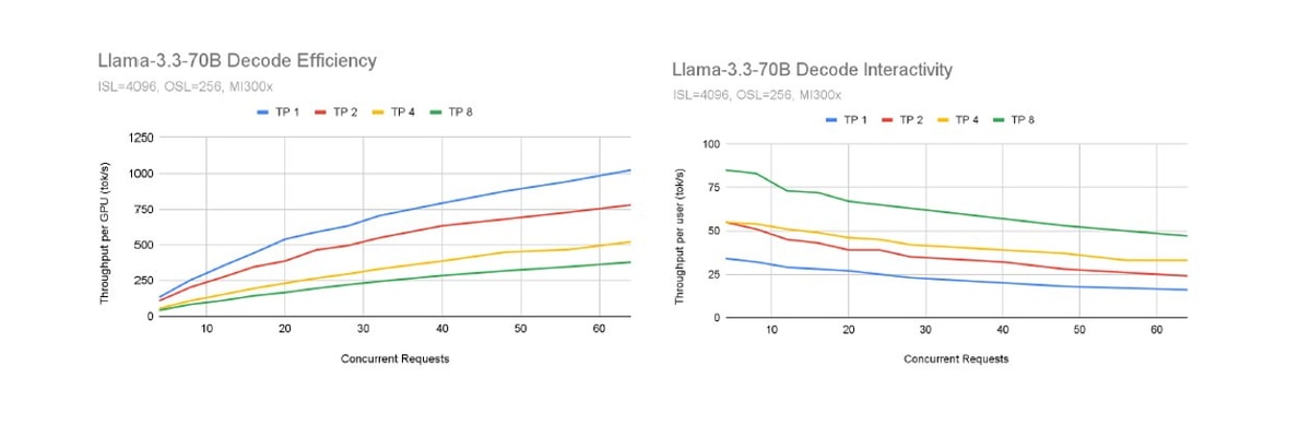
Efficiency per-GPU is not the only important metric to consider when deciding how to configure a vLLM server. Below are three graphs showing the interactivity and efficiency as we vary the number of concurrent requests and the parallelism. Top-left: the efficiency increases with concurrency but decreases with parallelism. Top-right: The interactivity decreases with concurrency but increases with parallelism.

Bringing it together, there is a tradeoff between efficiency and interactivity. When configuring a deployment of vLLM, it’s important to maximize efficiency while still maintaining the interactivity SLO.

How to configure P/D: We’ve shown how the parallelization of the prefill and the decode instances of vLLM affect both interactivity and efficiency. To attain a certain level of throughput, we can replicate the number of prefill and decode instances and vary the tensor parallelism. Thus, there are already four variables to be tuned, but the optimal configuration also depends on the parameters of the workload, including the ISL and OSL.

A brute-force approach in determining a cost-efficient, yet performant, disaggregated deployment is prohibitively time consuming due the combinatorial explosion of configurations to test out. We instead propose a decoupled benchmarking approach.

For a given ISL/OSL pair, we independently measure the performance of prefill-only and decode-only configurations under a range of concurrencies. Such baselines are then used to pair specific prefill configurations with the decode scenarios they are capable of saturating. This data-driven matching ensures we can identify a subset of prefill configurations that can provide tokens at a rate that maintains the target decode throughput.

We demonstrate how this methodology is applied to determine the optimal configurations for Llama-3.3-70B and gpt-oss-120b models when varying replicas count and tensor parallelism sizes for both prefill and decode inference phases. While we focus on Tensor-Parallel (TP) deployments exclusively, the method remains generally applicable to other scaling strategies.

Given ISL=4096 and OSL=256,

• First, we establish a baseline by running aggregated configuration sweeps over tensor parallel sizes 1,2,4,8 and a spread of concurrencies ranging from 4 to 64.
• Second, we evaluate disaggregated configurations by independently running prefill (ISL=4096) and decode (OSL=256) sweeps over tensor parallel sizes 1,2,4,8 and various concurrencies.

From the disaggregated prefill benchmarks, we identify the prefill throughput and at each concurrency level, we estimate the number of prefill instances required to sustain a decode instance.

Note: the execution of prefill and decode phases are completely decoupled by respectively setting OSL=1 and synthetically generating inputs of ISL size for the decode phase. This allows the user to easily deploy and execute independent vLLM PD configuration instances on a set of machines without requiring RDMA-enabled setups.

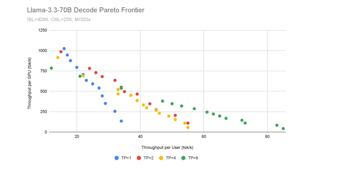
To evaluate the performance tradeoffs between aggregated and disaggregated configurations, we plot Throughput per GPU in (TPSG) against Throughput per User (TPSU). TPSU, measured in tokens per second per user, represents the interactivity of the system; how responsive it feels to individual users. TPSG, measured in tokens per second per GPU, captures infrastructure efficiency; how much work each GPU is doing. The higher the TPSG at some TPSU the better.

Figure 4 and 5 show the results of the configuration sweeps. TPSU is derived directly from concurrency. For disaggregated, TPSG is estimated by picking the prefill instance that performed best at that concurrency.

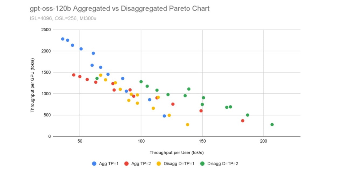
From figure 4, we see D=TP=2 emerging as a clear winner in certain TPSU (interactivity) ranges. In Table 2 (Appendix), refer to the column `Best P_GPUs`. Here, at all concurrencies, we see Prefill instances at TP=1 being sufficient to sustain the Decode TP=2 instance. This lets us read off column `Best P_GPUs` to provide the number of Prefill instances that seem promising.

With this, we generate the following disaggregated deployment candidates for further experiments,

1. 1p-tp1-1d-tp2 (1 prefill instance at TP=1, 1 decode instance at TP=2) - 3 GPUs
2. 2p-tp1-1d-tp2 (2 prefill instances at TP=1, 1 decode instance at TP=2) - 4 GPUs
3. 3p-tp1-1d-tp2 (3 prefill instances at TP=1, 1 decode instance at TP=2) - 5 GPUs

We perform the same experiment for the Llama-3.3-70B model.

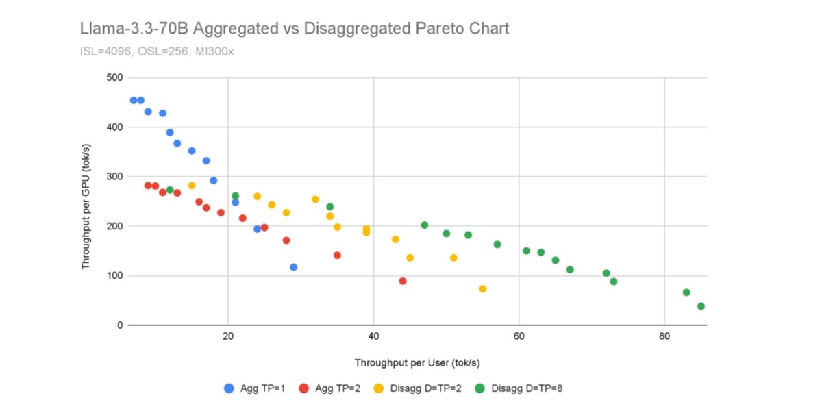
Targeting what seems to be the winning TPSU region (23 to 50), here we chose the candidates,

1. 1p-tp1-1d-tp2 (1 prefill instance with TP=1, 1 decode instance with TP=2) - 3 GPUs
2. 2p-tp1-1d-tp2 (2 prefill instance with TP=1, 1 decode instance with TP=2) - 4 GPUs
3. 3p-tp1-1d-tp2 (3 prefill instance with TP=1, 1 decode instance with TP=2) - 5 GPUs

We did not consider D=TP=8, despite the graph showing better performance in the high TPSU range as it has not scaled well based on our past experience. An interesting future work is to deep-dive into the observed discrepancy between the PD configs and Scaling experiments for D=TP=8.

Pareto Sweep

Code: j-pareto/pareto

The PD Configuration experiments gave us a principled way to identify promising disaggregated deployment candidates by analyzing prefill and decode phases in isolation. The Pareto Sweep experiments focus on end-to-end execution with real request flows. We benchmark both aggregated deployments (TP=1, TP=2, TP=4, TP=8) and our selected disaggregated deployment candidates (1p-tp1-1d-tp2, 2p-tp1-1d-tp2,3p-tp1-1d-tp2) across a wide range of concurrencies: 4, 8, 12, 16, 20, 24, 28, 32, 40, 48, 56, 64, 80, 96, 112, 128, 192, 256, 384, and 512.

This comprehensive sweep reveals where disaggregation actually delivers on its promise in production-like conditions, and which configurations dominate the efficiency frontier at different load levels.

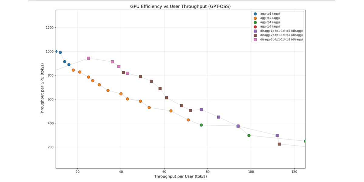
Figure 6 shows the resulting pareto frontier for both aggregated and disaggregated deployments. The disaggregated prefill-decode architecture demonstrates clear advantages in the TPSU regime (20-60 tok/s) by achieving superior GPU efficiency, delivering up to 600-950 tok/s per GPU compared to 500-800 tok/s for aggregated deployments at equivalent per-user throughput levels. This efficiency gain translates directly to cost savings: to serve the same number of users at similar latency guarantees (e.g., 60 tok/s per user), disaggregated deployments require fewer total GPUs, reducing operational expenses. However, aggregated deployments retain advantages at the extremes: at low TPSU (<20 tok/s), where the simplicity of unified instances reduces overheads, and at high TPSU (>100 tok/s), where aggressive tensor parallelism (TP=8) can serve latency-critical applications that require maximum per-user throughput regardless of efficiency considerations.

It is also interesting to note the fundamental trade-off between prefill capacity and utilization efficiency under different concurrency levels. At low concurrency (high TPSU, 80-120 tok/s), fewer requests are in-flight simultaneously. With a single prefill instance (1p-tp1-1d-tp2), high utilization is maintained by continuously processing available requests. Adding more prefill instances in this regime would result in under-utilization, reducing overall TPSG. Conversely, at high concurrency (low TPSU, 20-60 tok/s), many requests are in-flight simultaneously, creating a deeper queue of requests awaiting prefill. Here, the three prefill instance configuration (3p-tp1-1d-tp2) excels because multiple requests can be pulled and processed in parallel across the three instances.

The trade-off is clear: over-provisioning prefill capacity at low concurrency wastes GPU cycles on idle instances, while under-provisioning at high concurrency creates a prefill bottleneck that limits how many decode instances can be kept busy. This interplay between prefill instances, decode instances, and concurrency levels suggests that optimal disaggregated deployments require careful capacity planning or dynamic resource allocation.

We perform the same end-to-end sweep for Llama-3.3-70B to understand how disaggregation benefits translate across different model architectures.

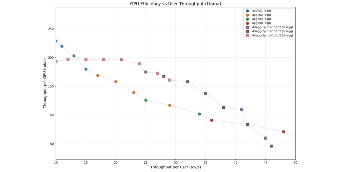
Figure 7 presents the resulting pareto frontier for both aggregated and disaggregated deployments of Llama-3.3-70B. We observe similar results to gpt-oss-120b where extremes are better suited to aggregated configurations while the mid-range interactivity favors disaggregated configurations. In the TPSU range of 15-41 tok/s, disaggregated configurations consistently deliver 10-38% higher throughput per GPU than aggregated deployments. At TPSU 25 tok/s, the disagg-2p-tp1-1d-tp2 configuration achieves 38% higher TPSG than the agg-tp4 configuration at the same GPU count.

Similar to the gpt-oss-120b results, we see a tradeoff between the number of prefill instances and TPSG in the targeted TPSU region; more prefill instances help at higher concurrency, while fewer suffice at lower concurrency levels.

Scale out

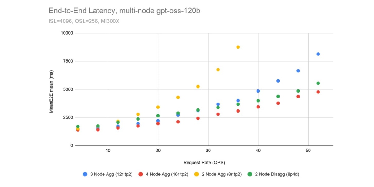
Finally, we scale out gpt-oss-120b aggregated configurations to a multi-node llm-d deployment to compare multi-node aggregated deployments to a 2 node disaggregated setup. The aggregated deployments all use tensor parallel size 2, and the disaggregated deployment uses eight prefill instances at TP=1 and four decode instances at TP=2, sweeping over request rates from 0 to 55 queries per second (QPS). In figure 8, we can observe that at low request rates, the 2 node disaggregated deployment behaves similarly to a 2 node aggregated one, but at higher request rates, the 2 node disaggregated deployment is faster than even a 3 node aggregated setup, showing how disaggregation leads to cheaper inference.

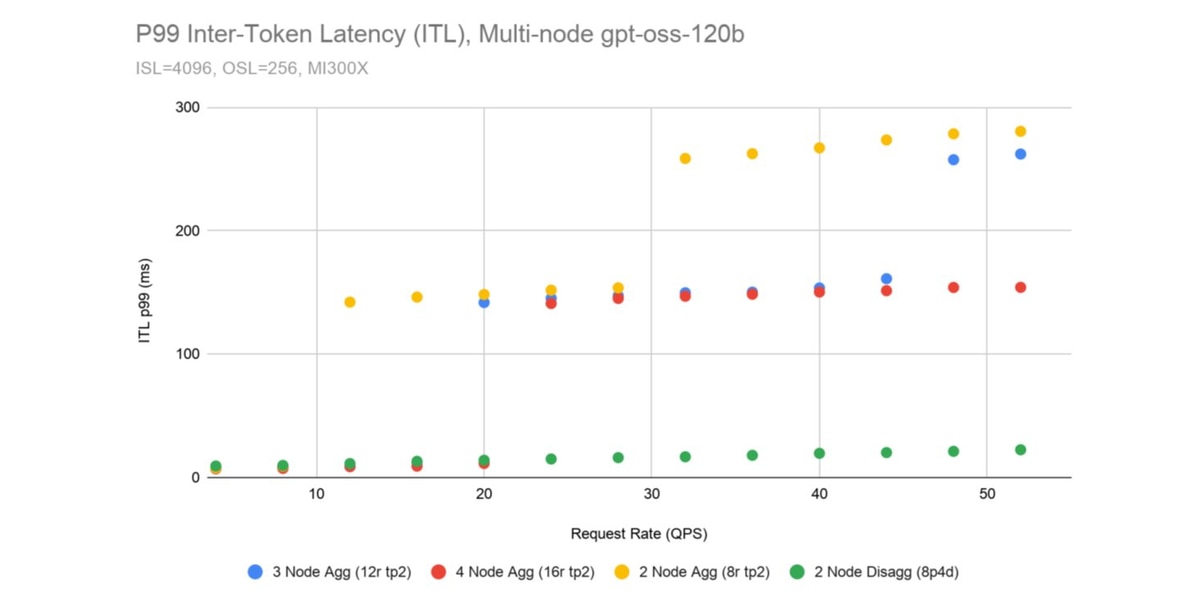
Another benefit of disaggregation is a large improvement to P99 inter-token latency. Separating prefill and decode solves a scheduling problem. In vLLM, chunked prefill allows prefill and decode iterations to co-mingle. This lets prefill and decode workloads to progress at each engine step but can lead to uneven token generation. In contrast, a P/D deployment has smooth token generation as the tokens being generated never have to wait for a long prefill step. Figure 9 shows the P99 inter-token latency achieved by aggregated and disaggregated deployments and how the 2 node disaggregated deployment stays low as the request rate increases above 20 queries per second.

Conclusion

This work demonstrates that prefill-decode disaggregated serving with llm-d provides a systematic pathway to optimize inference SLOs on the AMD MI300X infrastructure. The Pareto sweep analysis shows that in the mid-range interactivity regime, disaggregated architectures consistently have higher GPU efficiency compared to aggregated deployments, translating directly to reduced operational costs for enterprise LLM serving. Additionally, the scale-out experiment confirms these benefits extend to multi-node deployments where a lower node count disaggregated setup can outperform aggregated configurations at higher request rates while maintaining lower P99 inter-token latency. Our results highlight that optimal disaggregated deployment requires careful capacity planning. Through our decoupled benchmarking methodology, we provide practitioners with a repeatable workflow to identify the most efficient prefill-decode configuration for their specific model, workload, and SLO requirements, ultimately enabling teams to deliver better inference performance at lower infrastructure costs.

References

1. https://github.com/llm-d/llm-d
2. https://rocm.blogs.amd.com/artificial-intelligence/quick-reduce/README.html