Propelling Aerospace Innovation: Scaling Quantum Workflows on AMD Gpus With Rolls-Royce and Xanadu

Mar 10, 2026

Quantum hardware is advancing rapidly, but often faces the question: what is it actually useful for? To truly unlock the potential of quantum computing, we need not only to develop quantum algorithms to solve real, valuable, industrial problems, but also to build a scalable software stack that supports design today and execution tomorrow.

PennyLane, an open-source quantum software platform by Xanadu — a leading photonic quantum computing company — enables the design, compilation, and realization of meaningful quantum algorithms alongside the realities of quantum hardware. In a previous blog post, we explored how you can fast-track quantum simulation with Xanadu’s PennyLane on AMD GPUs. Today, we’ll look at how Xanadu and PennyLane are driving development of practical quantum algorithms with industry partners alongside AMD hardware.

One company that is exploring the potential of quantum computing is Rolls-Royce. For Rolls-Royce specifically, designing the next generation of efficient, low-emission jet engines relies heavily on simulating computational fluid dynamics (CFD) to model how air flows through the engine. These simulations involve solving massive systems of linear equations — a task that can consume vast amounts of classical supercomputing time for the largest simulations. Luckily, there is a leading candidate for solving these linear systems faster on fault-tolerant quantum computers (FTQC) — QSVT.

Below, we will outline the technical approach behind designing practical quantum algorithms for jet engine design, how the PennyLane software stack is used, and the performance results of this collaboration between Xanadu, AMD, and Rolls-Royce.

What is QSVT

Quantum computers are universal — anything we can compute classically, we can compute on quantum hardware. However, to achieve the potential speedups promised by quantum computing, we need quantum algorithms specially designed to exploit mathematical structure and interference to amplify correct solutions and cancel out incorrect ones, drastically reducing the computational steps required.

The Quantum Singular Value Transform (QSVT) algorithm is a cornerstone algorithm (sometimes referred to as providing a ‘grand unification’ of quantum algorithms) that enables the arbitrary transformation of a matrix via some specified polynomial, without the need to explicitly compute singular values. Remarkably, assuming we are able to encode the matrix on the quantum computer efficiently (that is, the quantum circuit for embedding the matrix scales polynomially in depth with matrix size), the entire computation will run in polynomial time.

Another advantage of the QSVT algorithm is that, while it generates deep quantum circuits (and thus will require fault-tolerant quantum computers (FTQC) with logical, error-corrected qubits), it requires a relatively small number of qubits, making it a promising algorithm for first-generation FTQC.

All of this makes QSVT a leading candidate for solving linear systems of equations on quantum computers, in a more scalable manner — exactly what Rolls-Royce is looking for to accelerate CFD modelling.

How Does This Apply to Fluid Dynamics?

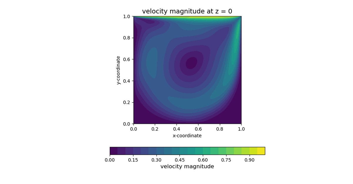
To be able to bridge the gap between next-generation jet engine design and quantum computing with QSVT, we need to first model the jet engine dynamics using CFD, before embedding a representation of that CFD model to solve with QSVT. For that first step, the Rolls-Royce team has generated various meshes representing a 2-dimensional lid-driven cavity test case. These meshes are represented as square matrices of increasing size, depending on the model's accuracy. From here, the non-linear fluid equations for laminar flow on this mesh are linearized — resulting in a large, sparse matrix with structure, but typically non-Hermitian.

Now that we have a large system of linear equations, the next step is to prepare the quantum computer to solve this via QSVT. This involves two steps:

Firstly, we need to efficiently embed this matrix in the quantum computer. We can take advantage of the sparse structure to improve embedding efficiency, and there are various available methods to doing this.
Secondly, we need to provide parameters (the phase angles) to the QSVT algorithm to perform the correct polynomial transformation of the matrix. Since we wish to solve a system of linear equations, we will need to encode a polynomial that inverts this matrix.

QSVT with Xanadu’s PennyLane

Thankfully, PennyLane makes both of these steps easy, with built-in functionality for QSVT and block encoding. Let’s walk through a simple example, showing how to apply a polynomial transformation to an input matrix, A.

		import numpy as np
import scipy as sp
from numpy.linalg import matrix_power as powm

A = np.array([
       [0.65713691, -0.05349524, 0.08024556, -0.07242864],
       [-0.05349524, 0.65713691, -0.07242864, 0.08024556],
       [0.08024556, -0.07242864, 0.65713691, -0.05349524],
       [-0.07242864, 0.08024556, -0.05349524, 0.65713691]])

The transformation we wish to apply is f (A) = 3 sin (A) exp (-A²) / 5. As this is not a polynomial, we will first need to find a polynomial approximation:

		def f(A):
   if isinstance(A, np.ndarray) and A.ndim == 2 and A.shape[0] == A.shape[1]:
       return 0.6 * sp.linalg.sinm(A) * sp.linalg.expm(-powm(A, 2))

   return 0.6 * np.sin(A) * np.exp(-A ** 2)

D = 15  # set the degree of the approximation
poly = np.round(sp.interpolate.approximate_taylor_polynomial(f, 0, D, 1), 7)

We can now begin the process of creating the QSVT quantum circuit to represent this transformation. First, we must generate the quantum operations to embed our matrix A into the quantum computer. One way of doing this is via the PrepSelPrep operation, which utilizes a technique known as Linear Combination of Unitaries (LCUs):

		import pennylane as qp
# represent the matrix as a Hamiltonian of Pauli terms on wires 3 and 4
H = qp.map_wires(qp.pauli_decompose(A), {0:3, 1: 4})
# use LCU method to encode this Hamiltonian
block_encode = qp.PrepSelPrep(H, control=[1, 2])

Next, we can use PennyLane’s poly_to_angles function to automatically generate the phase angle parameters that encode our polynomial transformation:

		angles = qp.poly_to_angles(poly[::-1], "QSVT")

We now have all the pieces to create our QSVT circuit, which can run on a quantum simulator or hardware device. Here, we choose to use PennyLane’s Lightning AMDGPU simulator, and utilize PennyLane’s built in PCPhase operation to encode the polynomial angles as quantum operations, and the QSVT operation to set up our QSVT algorithm.

		dev = qp.device("lightning.amdgpu")

@qp.qnode(dev)
def circuit(angles, init_state=None):

   if init_state is not None:
       # optionally embed an initial state to transform by f(A)
       qp.StatePrep(init_state, wires=[3, 4])

   projectors = [qp.PCPhase(a, dim=4, wires=[1, 2, 3, 4]) for a in angles]

   qp.Hadamard(0) # create a superposition state on our control wire
   qp.ctrl(qp.QSVT, control=0, control_values=[1])(block_encode, projectors)
   qp.ctrl(qp.adjoint(qp.QSVT), control=0, control_values=[0])(block_encode, projectors)
   qp.Hadamard(0)

   return qp.state()

Note that this quantum circuit is returning a quantum state — while this is possible on simulators and a useful tool for this tutorial, on hardware devices we would want to instead sample via qp.sample() and use statistical analysis to reconstruct the state. For more details on how this circuit works and its structure, check out the PennyLane Codebook chapter on QSVT.

Let’s now extract the matrix transformation that our quantum circuit is applying, to see if it is correctly applying our polynomial — we can use the matrix function to view the matrix transformation of the quantum circuit:

		matrix = qp.matrix(circuit, wire_order=range(5))(angles)
qsvt_A = np.round(matrix[:4, :4], 4).real

Comparing this to our expected transformation, we can see the error due to the polynomial approximation and the quantum circuit embedding:

		>>> np.linalg.norm(qsvt_A - f(A))
np.float64(0.05132140696322833)

A reasonably close approximation for our simple example! By increasing the accuracy of the polynomial approximation and utilizing different block encoding and circuit construction techniques, we could further increase the accuracy at the expense of deeper (and more expensive) quantum circuits.

Solving linear equations with QSVT

With a small tweak, we can extend this example to explore how to use the QSVT algorithm to solve a series of linear equations! Let’s solve the system , Ax = b where is given by the following vector:

		b = np.array([0.18257419, 0.36514837, 0.54772256, 0.73029674])

To solve this equation, we can invert the equation x = A^{- 1}b ; therefore, we would like to apply the transformation f (x) = 1/x to the matrix . Due to constraints in the QSVT algorithm, which requires polynomial transformations to be bounded in value between f ∈ [ -1,1] , we need to scale this equation, and so we will instead apply f(x) = s/x for some specified value . We can download a set of phase angles previously generated for s = 0.1 (K = 5) from the PennyLane Datasets service:

		[dataset] = qp.data.load("other", name="inverse")
inv_angles = dataset.angles["qsvt"]["0.001"]["5"]
s = 1 / (2*5)

We can now use the same circuit function as above to apply QSVT to solve this system of linear equations; we will use these new phase angles, as well as provide as an initial state to be embedded in the quantum system:

		output = circuit(inv_angles, init_state=b)

The solution to the linear equations will be encoded in the first 4 values. We will also divide the result by S to recover our original 1/x transformation, and normalize the result:

		output = np.round(output.real, 7)[:4] / s
output = output / np.linalg.norm(output)
array([0.20508119, 0.33462899, 0.58236358, 0.71191138])

How does this compare to the actual solution? We can normalize the actual solution to make a comparison:

		soln = np.linalg.solve(A, b)
soln = soln / np.linalg.norm(soln)
array([0.20539462, 0.33532754, 0.58192117, 0.71185409])

The solution to the equation agrees with the solution from the QSVT algorithm, with only small deviations!

		>>> np.linalg.norm(output - soln)
0.0008861224130015131

QSVT at scale

Now that we have explored how the QSVT algorithm works, let’s explore how this collaboration unlocked QSVT at scale for Rolls-Royce on AMD GPUs.

Recall that the QSVT algorithm requires two ingredients: a matrix representing a system of linear equations to be embedded, and a collection of phase angles representing a transformation on that matrix.

For that first ingredient, the Rolls-Royce team generated various meshes representing a 2-dimensional lid-driven cavity test case, and used this to generate a matrix representing laminar flow:

Contours of velocity magnitude at each position in the 256 x 256 CFD mesh.

Unlike in our simple example above using the LCU method to encode our matrix, for this more complicated matrix we utilize a bespoke embedding that takes advantage of the matrices’ -diagonal sparse structure.

For the phase angles representing the polynomial transformation needed to invert this matrix, a GPU compatible version of the Non-linear Fast Fourier Transform was implemented in PennyLane, which allows fast conversion of the inverse polynomial approximation into quantum operations.

With these two pieces in place, and leveraging the scalable infrastructure of Catalyst and Lightning, a 256 x 256 CFD matrix on 20 qubits with 35 million gates was compiled and executed on an AMD Instinct™ MI300X GPU in under two hours — a problem size that has never before been executed in a quantum setting.

Conclusion

While the power of quantum computing will be truly unlocked when FTQC hardware is here, for now, quantum simulation still plays an important role in validating quantum algorithm research. The results we shared here utilized a single GPU, but there is potential for scaling to even larger system sizes by distributing across multiple GPUs.

It is important to emphasize that even when FTQC is ready and available, we will still need to leverage classical computers to compile quantum programs for execution — for large circuits, this could require massive processing power. As a result, we need to continue scaling quantum software infrastructure to push the limits of compilation and simulation, making use of leading classical accelerator hardware and guided by practical applications in industry.

The path to quantum advantage is not a solo journey. It requires the industrial context of partners like Rolls-Royce, the hardware leadership of AMD, and the software ecosystem of PennyLane to connect the two — providing the software stack that allows researchers to express complex algorithms like QSVT and compile them for high-performance execution. If you are interested in learning more or have any follow-up questions, reach out to quantum@amd.com.

Other Resources

Expanding the Frontier: Learn how PennyLane and AMD accelerate quantum workflows
PennyLane documentation - Full guides, tutorials, and API reference
Xanadu YouTube Channel - Watch hands-on tutorials and deep dives into PennyLane features.
AMD Developer Cloud - Start projects on AMD Instinct™ GPUs
The PennyLane Guide to Hamiltonian Simulation - An overview of QSVT
QSVT for Hamiltonian Simulation - An interactive textbook with theory and coding exercises
QSVT in Practice – Explore in more detail the usage of QSVT to solve systems of linear equations